Now that I can graph ASM performance metrics, let’s see some use cases.
To display the ASM metrics I’ll use the csv file generated by the csv_asm_metrics utility and Tableau for the visualization. Of course you could use the visualization tool of your choice.
Use case 1: Display the TOP IO consumers
You consolidated several databases on the same machine and you want to visualize which database is generating most of the IO throughput for Reads. You can visualize this that way with Tableau (I keep the “columns”, “rows” and “marks” shelf into the print screen so that you can reproduce with Tableau) :
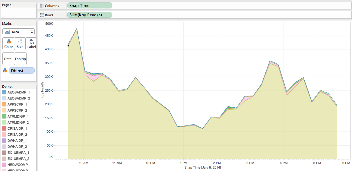
I can see that one of my databases is generating most of the throughput.
Should you use RAC, you could split those metrics per ASM instances as well:
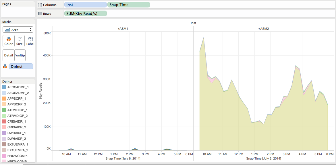
I can see that most of the activity is recorded on ASM2, which makes sense as my RAC services are configured as preferred/available (Active/Passive configuration) and started on the *_2 database instances (linked to ASM2).
Use case 2: I want to see the Read IO distributions by Failgroups
You can visualize this that way with Tableau (I keep the “columns”, “rows” and “marks” shelf into the print screen so that you can reproduce with Tableau):
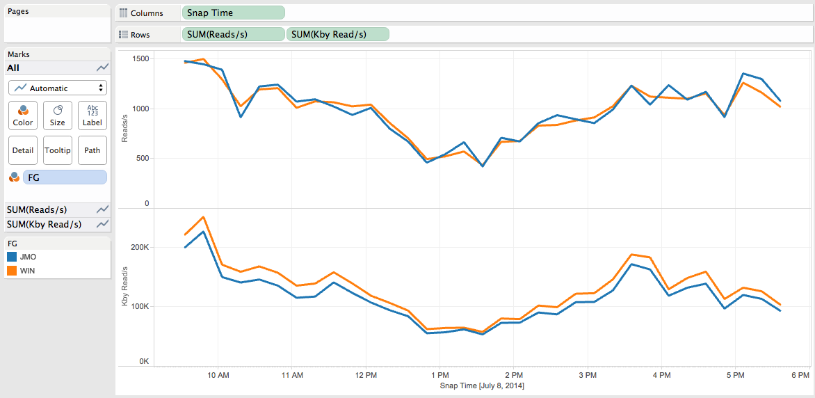
We can see that the IOs are equally distributed over the Failgroups. It is the expected behaviour as I am not using the ASM Preferred Read feature.
Use case 3: Should I use the ASM Preferred Read feature on my extended RAC?
Suppose the host hosting the ASM1 instance is close to the disk array on which the “WIN” failgroup has been created. The same way, the host hosting the ASM2 instance is close to the disk array on which the “JMO” failgroup has been created. Let’s see the Read IO latency between the ASM instances and the failgroups.
You can visualize this that way with Tableau (I keep the “columns”, “rows” and “marks” shelf into the print screen so that you can reproduce with Tableau):
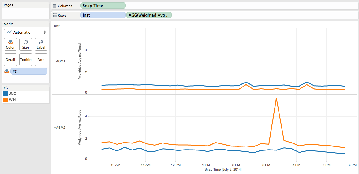
As you can see the ASM1 instance reports faster reads on the “WIN” failgroup and ASM2 reports faster reads on the “JMO” failgroup which makes sense according to our configuration. I can also check if the reads performance are good enough when the Reads are done on the farthest disk array (ASM1 “reading” on the JMO failgroup and ASM2 “reading” on the WIN failgroup) and then decide if the ASM Preferred Read feature needs to be implemented.
Use case 4: Simulate and Visualize the impact of the ASM preferred feature on the read IOPS and throughput (See this blog post).
Use case 5: Are ASM rebalance and preferred read working together? (See this blog post)
Use case 6: A closer look at ASM rebalance, Part I: Disks have been added. (See this blog post)
Use case 7: A closer look at ASM rebalance, Part II: Disks have been dropped. (See this blog post)
Use case 8: A closer look at ASM rebalance, Part III: Disks have been added and dropped (at the same time). (See this blog post)
Remarks:
- ASM is not performing any reads for the database, it records metrics for the database instances that it is servicing.
- I am not using the Flex ASM feature for the previous use cases. With the Flex ASM feature in place the interpretations done into the use case 3 would not have been possible (as ASM1 could serve database instance located near to ASM2 and vice versa). Furthermore the preferred read feature is broken with Flex ASM 12c (12.1) in place.
- You can imagine a lot of use cases thanks to the measures collected (Reads/s, Kby Read/s, ms/Read, By/Read, Writes/s, Kby Write/s, ms/Write, By/Write) and all those dimensions (Snap Time, INST, DBINST, DG, FG, DSK).
- Don’t forget that If you don’t picture it, you may not understand it.
You can download the asm_metrics and the csv_asm_metrics utilities from this repository.