ASM metrics are a goldmine, they provide a lot of informations. As you may know, the asm_metrics utility extracts them in real-time.
But sometimes it is not easy to understand the values without the help of a graph. Look at this example: If I cant’ picture it, I can’t understand it.
So depending on your needs, depending on what you are looking for with the ASM metrics: A picture may help.
So let’s graph the output of the asm_metrics utility: For this I created the csv_asm_metrics utility to produce a csv file from the output of the asm_metrics utility.
Once you get the csv file you can graph the metrics with your favourite visualization tool (I’ll use Tableau as an example).
First you have to launch the asm_metrics utility that way (To ensure that all the fields are displayed):
- -show=inst,dbinst,fg,dg,dsk for ASM >= 11g
- -show=inst,fg,dg,dsk for ASM < 11g
and redirect the output to a text file:
./asm_metrics.pl -show=inst,dbinst,fg,dg,dsk > asm_metrics.txt
Remark: You can use the -interval parameter to collect data with an interval greater than one second (the default interval), as it could produce a huge output file.
The output file looks like:
............................
Collecting 1 sec....
............................

......... SNAP TAKEN AT ...................

13:48:54                                                                              Kby       Avg       AvgBy/               Kby       Avg        AvgBy/
13:48:54   INST     DBINST        DG            FG           DSK            Reads/s   Read/s    ms/Read   Read      Writes/s   Write/s   ms/Write   Write
13:48:54   ------   -----------   -----------   ----------   ----------     -------   -------   -------   ------    ------     -------   --------   ------
13:48:54   +ASM1                                                            6731      54224     1.4       8249      42         579       3.0        14117
13:48:54   +ASM1    BDT10_1                                                 2         32        0.2       16384     0          0         0.0        0
13:48:54   +ASM1    BDT10_1       DATA                                      2         32        0.2       16384     0          0         0.0        0
13:48:54   +ASM1    BDT10_1       DATA          HOST31                      0         0         0.0       0         0          0         0.0        0
13:48:54   +ASM1    BDT10_1       DATA          HOST31       HOST31CA0D1C   0         0         0.0       0         0          0         0.0        0
13:48:54   +ASM1    BDT10_1       DATA          HOST31       HOST31CA0D1D   0         0         0.0       0         0          0         0.0        0
13:48:54   +ASM1    BDT10_1       DATA          HOST32                      2         32        0.2       16384     0          0         0.0        0
13:48:54   +ASM1    BDT10_1       DATA          HOST32       HOST32CA0D1C   0         0         0.0       0         0          0         0.0        0
13:48:54   +ASM1    BDT10_1       DATA          HOST32       HOST32CA0D1D   2         32        0.2       16384     0          0         0.0        0
13:48:54   +ASM1    BDT10_1       FRA                                       0         0         0.0       0         0          0         0.0        0
13:48:54   +ASM1    BDT10_1       FRA           HOST31                      0         0         0.0       0         0          0         0.0        0
13:48:54   +ASM1    BDT10_1       FRA           HOST31       HOST31CC8D0F   0         0         0.0       0         0          0         0.0        0
13:48:54   +ASM1    BDT10_1       FRA           HOST32                      0         0         0.0       0         0          0         0.0        0
13:48:54   +ASM1    BDT10_1       FRA           HOST32       HOST32CC8D0F   0         0         0.0       0         0          0         0.0        0

and so on...
Now let’s produce the csv file with the csv_asm_metrics utility. Let’s see the help:
./csv_asm_metrics.pl -help

Usage: ./csv_asm_metrics.pl [-if] [-of] [-d] [-help]

  Parameter         Comment
  ---------         -------
  -if=              Input file name (output of asm_metrics)
  -of=              Output file name (the csv file)
  -d=               Day of the first snapshot (YYYY/MM/DD)

Example: ./csv_asm_metrics.pl -if=asm_metrics.txt -of=asm_metrics.csv -d='2014/07/04'
and generate the csv file that way:
./csv_asm_metrics.pl -if=asm_metrics.txt -of=asm_metrics.csv -d='2014/07/04'
The csv file looks like:
Snap Time,INST,DBINST,DG,FG,DSK,Reads/s,Kby Read/s,ms/Read,By/Read,Writes/s,Kby Write/s,ms/Write,By/Write
2014/07/04 13:48:54,+ASM1,BDT10_1,DATA,HOST31,HOST31CA0D1C,0,0,0.0,0,0,0,0.0,0
2014/07/04 13:48:54,+ASM1,BDT10_1,DATA,HOST31,HOST31CA0D1D,0,0,0.0,0,0,0,0.0,0
2014/07/04 13:48:54,+ASM1,BDT10_1,DATA,HOST32,HOST32CA0D1C,0,0,0.0,0,0,0,0.0,0
2014/07/04 13:48:54,+ASM1,BDT10_1,DATA,HOST32,HOST32CA0D1D,2,32,0.2,16384,0,0,0.0,0
2014/07/04 13:48:54,+ASM1,BDT10_1,FRA,HOST31,HOST31CC8D0F,0,0,0.0,0,0,0,0.0,0
2014/07/04 13:48:54,+ASM1,BDT10_1,FRA,HOST32,HOST32CC8D0F,0,0,0.0,0,0,0,0.0,0
2014/07/04 13:48:54,+ASM1,BDT10_1,REDO1,HOST31,HOST31CC0D13,0,0,0.0,0,0,0,0.0,0
2014/07/04 13:48:54,+ASM1,BDT10_1,REDO1,HOST32,HOST32CC0D13,0,0,0.0,0,0,0,0.0,0
2014/07/04 13:48:54,+ASM1,BDT10_1,REDO2,HOST31,HOST31CC0D12,0,0,0.0,0,0,0,0.0,0
2014/07/04 13:48:54,+ASM1,BDT10_1,REDO2,HOST32,HOST32CC0D12,0,0,0.0,0,0,0,0.0,0
2014/07/04 13:48:54,+ASM1,BDT11_1,DATA,HOST31,HOST31CA0D1C,0,0,0.0,0,0,0,0.0,0
2014/07/04 13:48:54,+ASM1,BDT11_1,DATA,HOST31,HOST31CA0D1D,0,0,0.0,0,2,16,0.5,8448
As you can see:
- The day has been added (to create a date) and next ones will be calculated (should the snaps cross multiple days).
- Only the rows that contain all the fields have been recorded into the csv file (The script does not record the other ones as they represent aggregated values).
Now I can import this csv file into Tableau.
You can imagine a lot of graphs thanks to the measures collected (Reads/s, Kby Read/s, ms/Read, By/Read, Writes/s, Kby Write/s, ms/Write, By/Write) and all those dimensions (Snap Time, INST, DBINST, DG, FG, DSK).
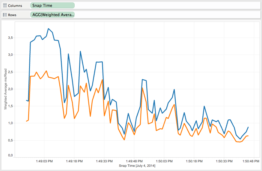
Let’s graph the throughput and latency per failgroup for example.
Important remark regarding some averages computation/display:
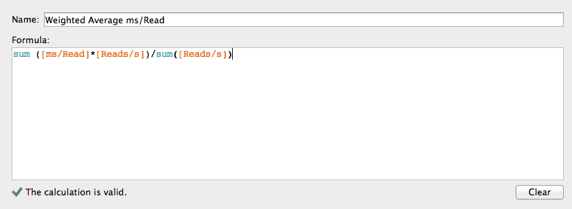
The ms/Read and By/Read measures depend on the number of reads. So the averages have to be calculated using Weighted Averages. (The same apply for ms/Write and By/Write).
Let’s create the calculated field in Tableau for those Weighted Averages:
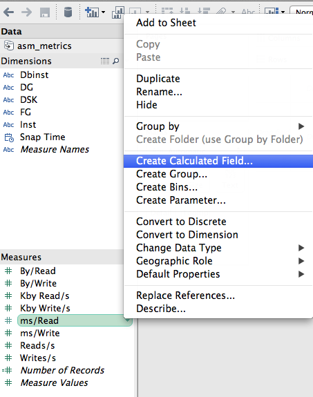
so that weighted Average ms/Read is:
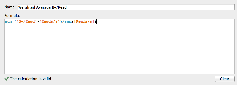
Weighted Average By/Read:
The same way you have to create:
- Weighted Average ms/Write = sum([ms/Write]*[Writes/s])/sum([Writes/s])
- Weighted Average By/Write = sum([By/Write]*[Writes/s])/sum([Writes/s])
Now let’s display the average read latency by Failgroup (using the previous calculated weighted average):
Drag the Snap Time dimension to the “columns” shelf and choose “exact date”:
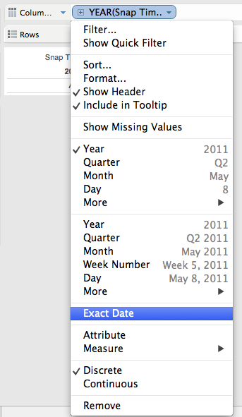
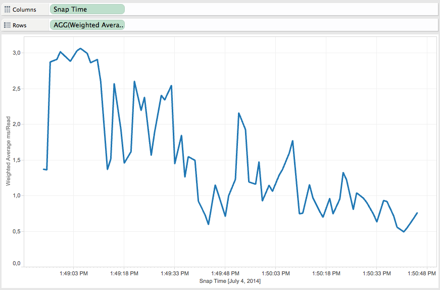
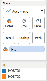
Here we are.
Conclusion:
- We can create a csv file from the output of the asm_metrics utility thanks to csv_asm_metrics.
-
To do so, we have to collect all the fields of asm_metrics with those options:
- -show=inst,dbinst,fg,dg,dsk for ASM >= 11g
- -show=inst,fg,dg,dsk for ASM < 11g
- Once you uploaded the csv file into your favourite visualization tool, don’t forget to calculate weighted averages for ms/Read, By/Read, ms/Write and By/Write if you plan to graph the averages.
- You can imagine a lot of graphs thanks to the measures collected (Reads/s, Kby Read/s, ms/Read, By/Read, Writes/s, Kby Write/s, ms/Write, By/Write) and all those dimensions (Snap Time, INST, DBINST, DG, FG, DSK).
You can download the csv_asm_metrics utility from this repository or copy the source code from this page.
UPDATE: You can see some use cases here.