As you know, the wait event “db file sequential read” records “single block” IO performed outside the database buffer cache. But does the IO come from:
- Filesystem cache (If any and used)
- Disk Array cache
- SSD
- Spindle Disks
- …..
It could be interesting to visualize the distribution of the IO source:
- Should you migrate from a cached filesystem to ASM (You may need to increase the database cache to put the previous Filesystem cached IOs into the database cache).
- Should you use Dynamic Tiering and want to figure out where the IOs come from (SSD, Spindle Disks..).
To do so, I’ll use the AWR data coming from the dba_hist_event_histogram view and Tableau. I’ll also extract the data coming from dba_hist_snapshot (to get the begin_interval_date time).
alter session set nls_date_format='YYYY/MM/DD HH24:MI:SS';
alter session set nls_timestamp_format='YYYY/MM/DD HH24:MI:SS';

select * from dba_hist_event_histogram where
snap_id >= (select min(snap_id) from dba_hist_snapshot
where begin_interval_time >= to_date ('2014/06/01 00:00','YYYY/MM/DD HH24:MI'))
and event_name='db file sequential read';

select * from dba_hist_snapshot where begin_interval_time >= to_date ('2014/06/01 00:00','YYYY/MM/DD HH24:MI');
As you can see, there is no computation. This is just a simple extraction of the data.
Then I put those data into 2 csv files (awr_snap_for_june.csv and awr_event_histogram.csv).
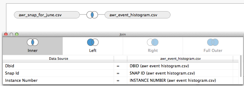
1) Now, launch Tableau and select the csv files and add an inner join between those files:
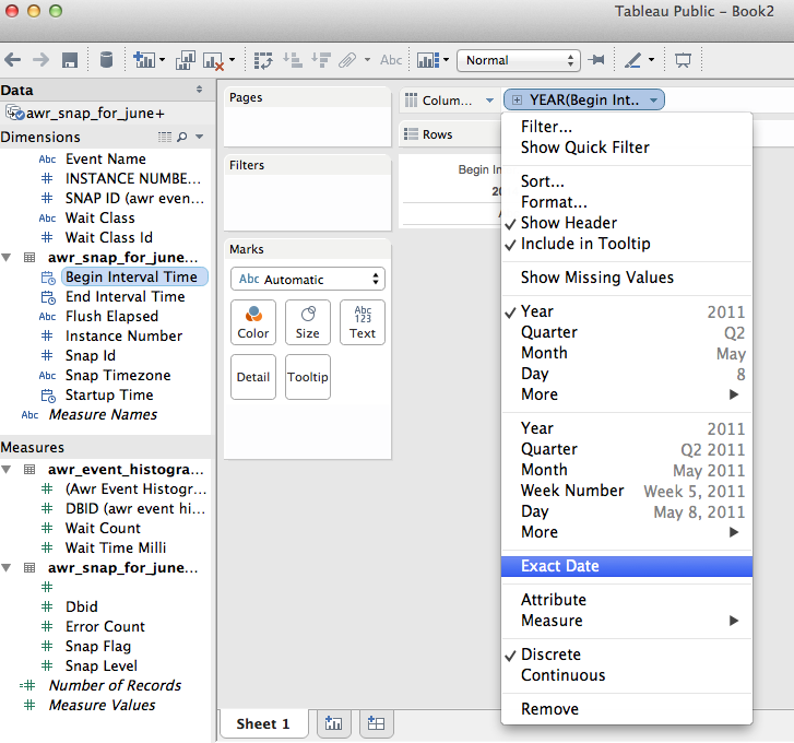
2) Go to the worksheet and put the “begin interval time” dimension into the “column” and change it to an “exact date” (Instead of Year):
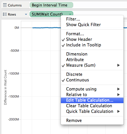
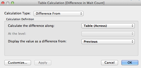
3) Put the “Wait count” measure into the “Rows” and create a table calculation on it:
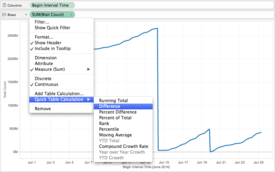
Choose “difference” as the “WAIT_COUNT” field is cumulative and we want to see the delta between the AWR’s snapshots.
4) My graph now looks like:
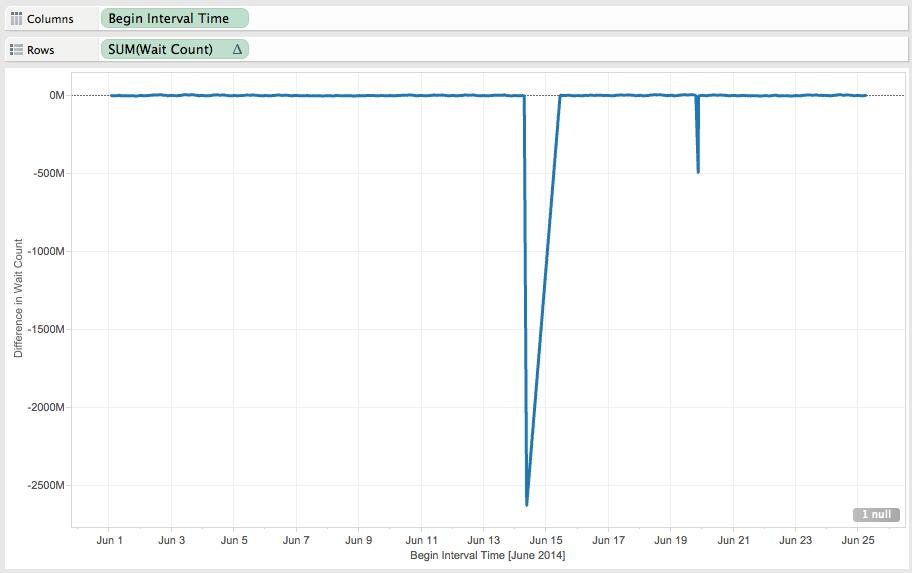
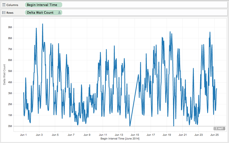
The Jun 14 and Jun 20 the database has been re-started and then the difference is < 0.
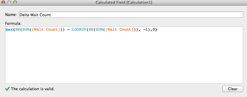
5) Let’s modify the formula to take care of database restart into the delta computation:
Customize
Name: “Delta Wait Count” and change ZN(SUM([Wait Count])) - LOOKUP(ZN(SUM([Wait Count])), -1) to max(ZN(SUM([Wait Count])) - LOOKUP(ZN(SUM([Wait Count])), -1),0):
So that now the graph looks like:
6) Now we have to “split” those wait count into 2 categories based on the wait_time_milli measure coming from dba_hist_event_histogram. Let’s say that:
- “db file sequential read” <= 4 ms are not coming from spindle disks (So from caching, SSD..).
- “db file sequential read” > 4 ms are coming from spindle disks.
Let’s implement this in tableau with a calculated field:
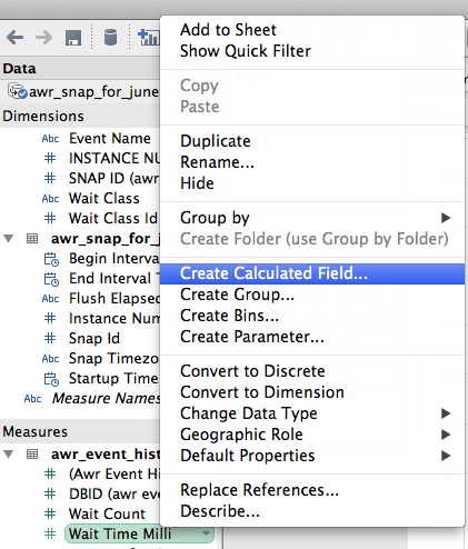
Name: “IO Source” and use this formula:
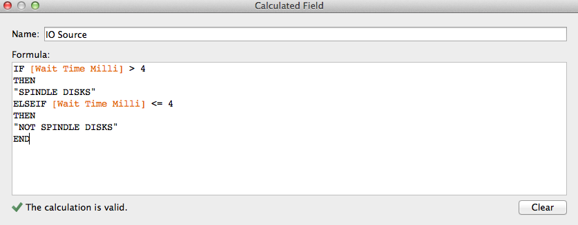
Feel free to modify this formula according to your environment.
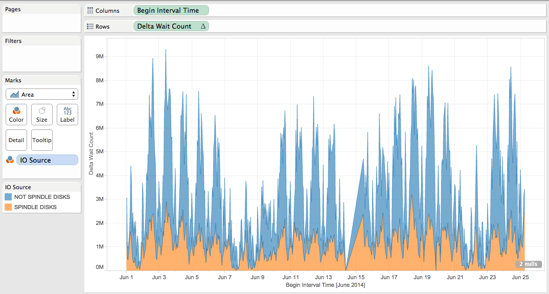
Now take the “IO Source” Dimension and put it into the Color marks:
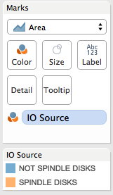
So that we can now visualize the IO source repartition:
Remarks:
- Karl Arao presented another example usage of Tableau into this blog post.
- Should you need to retrieve ”db file sequential read” buckets < 1 ms, then you can use oracle_trace_parsing from Kyle Hailey.
Update 1: Example of oracle_trace_parsing usage into “Oracle “Physical I/O” ? not always physical” blog post.
Update 2: Another way to retrieve “db file sequential read” buckets < 1 ms (With external tables this time) into Nikolay Savvinov blog post.