Extract Exadata cells historical metrics in CSV format

Exadata provides a lot of useful metrics to monitor the Cells and you may want to retrieve historical values for some metrics. To do so, you can use the “LIST METRICHISTORY” command through CellCLI on the cell.

But as usual, visualising the metrics is even more better. For this purpose, you can use a perl script (see the download link in the remarks section) that extracts the historical metrics in CSV format so that you can graph them with the visualisation tool of your choice.

Let’s see the help:

Usage: ./csv_exadata_metrics_history.pl [cell=|groupfile=] [serial] [type=] [name=] [objectname=] [name!=] [objectname!=] [ago_unit=] [ago_value=]

 Parameter                 Comment                                                      Default
 ---------                 -------                                                      -------
 CELL=                     comma-separated list of cells
 GROUPFILE=                file containing list of cells
 SERIAL                    serialize execution over the cells (default is no)
 TYPE=                     Metrics type to extract: Cumulative|Rate|Instantaneous       ALL
 NAME=                     Metrics to extract (wildcard allowed)                        ALL
 OBJECTNAME=               Objects to extract (wildcard allowed)                        ALL
 NAME!=                    Exclude metrics (wildcard allowed)                           EMPTY
 OBJECTNAME!=              Exclude objects (wildcard allowed)                           EMPTY
 AGO_UNIT=                 Unit to retrieve historical metrics back: day|hour|minute    HOUR
 AGO_VALUE=                Value associated to Unit to retrieve historical metrics back 1

utility assumes passwordless SSH from this cell node to the other cell nodes
utility assumes ORACLE_HOME has been set (with celladmin user for example)

Example : ./csv_exadata_metrics_history.pl cell=cell
Example : ./csv_exadata_metrics_history.pl groupfile=./cell_group
Example : ./csv_exadata_metrics_history.pl cell=cell objectname='CD_disk03_cell'
Example : ./csv_exadata_metrics_history.pl cell=cell name='.*BY.*' objectname='.*disk.*'
Example : ./csv_exadata_metrics_history.pl cell=enkcel02 name='.*DB_IO.*' objectname!='ASM' name!='.*RQ.*' ago_unit=minute ago_value=4
Example : ./csv_exadata_metrics_history.pl cell=enkcel02 type='Instantaneous' name='.*DB_IO.*' objectname!='ASM' name!='.*RQ.*' ago_unit=hour ago_value=4
Example : ./csv_exadata_metrics_history.pl cell=enkcel01,enkcel02 type='Instantaneous' name='.*DB_IO.*' objectname!='ASM' name!='.*RQ.*' ago_unit=minute ago_value=4 serial

You have to setup passwordless SSH from one cell to the other cells (Then you can launch the script from this cell and retrieve data from the other cells).

The main options/features are:

You can specify the cells on which you want to collect the metrics thanks to the cell or groupfile parameter.
You can choose to serialize the execution over the cells thanks to the serial parameter.
You can choose the type of metrics you want to retrieve (Cumulative, rate or instantaneous) thanks to the type parameter.
You can focus on some metrics thanks to the name parameter (wildcard allowed).
You can exclude some metrics thanks to the name! parameter (wildcard allowed).
You can focus on some metricobjectname thanks to the objectname parameter (wildcard allowed).
You can exclude some metricobjectname thanks to the objectname! parameter (wildcard allowed).
You can choose the unit to retrieve metrics back (day, hour, minute) thanks to the ago_unit parameter.
You can choose the value associated to the unit to retrieve metrics back thanks to the ago_value parameter.

Let’s see an example:

I want to retrieve in csv format the metrics from 2 cells related to databases for the last 20 minutes:

$> ./csv_exadata_metrics_history.pl cell=enkx3cel01,enkx3cel02 name='DB_.*' ago_unit=minute ago_value=20
Cell;metricType;DateTime;name;objectname;value;unit
enkx3cel01;Instantaneous;2015-07-01T08:57:59-05:00;DB_FC_BY_ALLOCATED;ACSTBY;0.000;MB
enkx3cel01;Instantaneous;2015-07-01T08:57:59-05:00;DB_FC_BY_ALLOCATED;ASM;15,779;MB
enkx3cel01;Instantaneous;2015-07-01T08:57:59-05:00;DB_FC_BY_ALLOCATED;BDT;0.000;MB
enkx3cel01;Instantaneous;2015-07-01T08:57:59-05:00;DB_FC_BY_ALLOCATED;BIGDATA;0.000;MB
enkx3cel01;Instantaneous;2015-07-01T08:57:59-05:00;DB_FC_BY_ALLOCATED;DBFS;0.000;MB
enkx3cel01;Instantaneous;2015-07-01T08:57:59-05:00;DB_FC_BY_ALLOCATED;DBM;15,779;MB
enkx3cel01;Instantaneous;2015-07-01T08:57:59-05:00;DB_FC_BY_ALLOCATED;DEMO;794,329;MB
enkx3cel01;Instantaneous;2015-07-01T08:57:59-05:00;DB_FC_BY_ALLOCATED;DEMOX3;0.000;MB
enkx3cel01;Instantaneous;2015-07-01T08:57:59-05:00;DB_FC_BY_ALLOCATED;EXDB;0.000;MB
enkx3cel01;Instantaneous;2015-07-01T08:57:59-05:00;DB_FC_BY_ALLOCATED;WZSDB;0.000;MB
enkx3cel01;Instantaneous;2015-07-01T08:57:59-05:00;DB_FC_BY_ALLOCATED;_OTHER_DATABASE_;48,764;MB
enkx3cel01;Instantaneous;2015-07-01T08:57:59-05:00;DB_FC_IO_BY_SEC;ACSTBY;0;MB/sec
enkx3cel01;Instantaneous;2015-07-01T08:57:59-05:00;DB_FC_IO_BY_SEC;ASM;0;MB/sec
enkx3cel01;Instantaneous;2015-07-01T08:57:59-05:00;DB_FC_IO_BY_SEC;BDT;0;MB/sec
enkx3cel01;Instantaneous;2015-07-01T08:57:59-05:00;DB_FC_IO_BY_SEC;BIGDATA;0;MB/sec
enkx3cel01;Instantaneous;2015-07-01T08:57:59-05:00;DB_FC_IO_BY_SEC;DBFS;0;MB/sec
enkx3cel01;Instantaneous;2015-07-01T08:57:59-05:00;DB_FC_IO_BY_SEC;DBM;15;MB/sec
enkx3cel01;Instantaneous;2015-07-01T08:57:59-05:00;DB_FC_IO_BY_SEC;DEMO;0;MB/sec
enkx3cel01;Instantaneous;2015-07-01T08:57:59-05:00;DB_FC_IO_BY_SEC;DEMOX3;0;MB/sec
enkx3cel01;Instantaneous;2015-07-01T08:57:59-05:00;DB_FC_IO_BY_SEC;EXDB;0;MB/sec
enkx3cel01;Instantaneous;2015-07-01T08:57:59-05:00;DB_FC_IO_BY_SEC;WZSDB;0;MB/sec
enkx3cel01;Instantaneous;2015-07-01T08:57:59-05:00;DB_FC_IO_BY_SEC;_OTHER_DATABASE_;0;MB/sec
enkx3cel01;Cumulative;2015-07-01T08:57:59-05:00;DB_FC_IO_RQ;ACSTBY;2,318;IO requests
enkx3cel01;Cumulative;2015-07-01T08:57:59-05:00;DB_FC_IO_RQ;ASM;0;IO requests
enkx3cel01;Cumulative;2015-07-01T08:57:59-05:00;DB_FC_IO_RQ;BDT;2,966;IO requests
enkx3cel01;Cumulative;2015-07-01T08:57:59-05:00;DB_FC_IO_RQ;BIGDATA;25,415;IO requests
enkx3cel01;Cumulative;2015-07-01T08:57:59-05:00;DB_FC_IO_RQ;DBFS;3,489;IO requests
enkx3cel01;Cumulative;2015-07-01T08:57:59-05:00;DB_FC_IO_RQ;DBM;1,627,066;IO requests
enkx3cel01;Cumulative;2015-07-01T08:57:59-05:00;DB_FC_IO_RQ;DEMO;4,506;IO requests
enkx3cel01;Cumulative;2015-07-01T08:57:59-05:00;DB_FC_IO_RQ;DEMOX3;4,172;IO requests
enkx3cel01;Cumulative;2015-07-01T08:57:59-05:00;DB_FC_IO_RQ;EXDB;0;IO requests
enkx3cel01;Cumulative;2015-07-01T08:57:59-05:00;DB_FC_IO_RQ;WZSDB;4,378;IO requests
enkx3cel01;Cumulative;2015-07-01T08:57:59-05:00;DB_FC_IO_RQ;_OTHER_DATABASE_;6,227;IO requests
enkx3cel01;Cumulative;2015-07-01T08:57:59-05:00;DB_FC_IO_RQ_LG;ACSTBY;0;IO requests
.
.
.

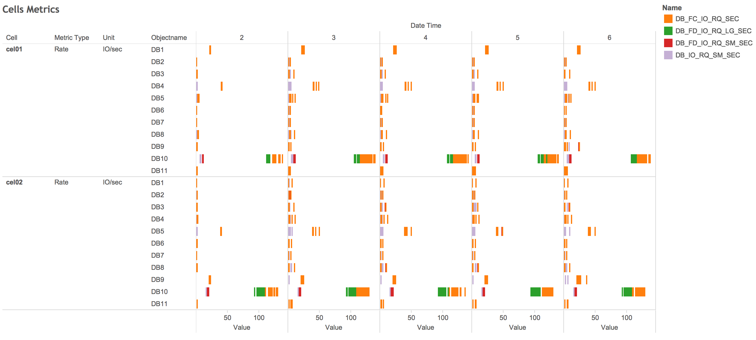
That way, you could visualize your data the way you feel comfortable with. For example, I used tableau to create this “Database metrics dashboard” on DB_* rate metrics:

cells_metrics

Remarks:

If you retrieve too much data, you could receive something like:

Error: enkx3cel02 is returning over 100000 lines; output is truncated !!!
 Command could be retried with the serialize option: --serial
 Killing child pid 15720 to enkx3cel02...

Then, you can launch the script with the serial option (see the help).

You can download the csv_exadata_metrics_history.pl script from this repository , or from Github.

Conclusion:

You probably already have a way to build your own graph of the historical metrics. But if you don’t, feel free to use this script and the visualisation tool of your choice.