Into my last post I gave a way to Retrieve and visualize wait events metrics from AWR with R, now it’s time for the system statistics.
So, for a particular system statistic, I’ll retrieve from the dba_hist_sysstat view:
- Its VALUE between 2 snaps
- Its VALUE per second between 2 snaps
As the VALUE is cumulative, I need to compute the difference between 2 snaps that way:
SQL> !cat check_awr_stats.sql
set linesi 200
col BEGIN_INTERVAL_TIME format a28
col stat_name format a40

alter session set nls_timestamp_format='YYYY/MM/DD HH24:MI:SS';
alter session set nls_date_format='YYYY/MM/DD HH24:MI:SS';

select s.begin_interval_time,sta.stat_name,sta.VALUE,
--round(((sta.VALUE)/(to_date(s.end_interval_time)-to_date(s.begin_interval_time)))/86400,2) VALUE_PER_SEC_NOT_ACCURATE,
round(((sta.VALUE)/
(
(extract(day from s.END_INTERVAL_TIME)-extract(day from s.BEGIN_INTERVAL_TIME))*86400 +
(extract(hour from s.END_INTERVAL_TIME)-extract(hour from s.BEGIN_INTERVAL_TIME))*3600 +
(extract(minute from s.END_INTERVAL_TIME)-extract(minute from s.BEGIN_INTERVAL_TIME))*60 +
(extract(second from s.END_INTERVAL_TIME)-extract(second from s.BEGIN_INTERVAL_TIME))
)
),2) VALUE_PER_SEC
from
(
select instance_number,snap_id,stat_name,
value - first_value(value) over (partition by stat_name order by snap_id rows 1 preceding) "VALUE"
from
dba_hist_sysstat
where stat_name like nvl('&stat_name',stat_name)
and instance_number = (select instance_number from v$instance)
) sta, dba_hist_snapshot s
where sta.instance_number=s.instance_number
and sta.snap_id=s.snap_id
and s.BEGIN_INTERVAL_TIME >= trunc(sysdate-&sysdate_nb_day_begin_interval+1)
and s.BEGIN_INTERVAL_TIME <= trunc(sysdate-&sysdate_nb_day_end_interval+1)
order by s.begin_interval_time asc;
I use the “partition by stat_name order by snap_id rows 1 preceding” to compute the difference between snaps par stat_name.
I also use Extract to get an accurate value per second, you should read this blog post to understand why.
The output is like:
SQL> @check_awr_stats.sql

Session altered.

Session altered.

Enter value for stat_name: physical reads
old  17: where stat_name like nvl('&stat_name',stat_name)
new  17: where stat_name like nvl('physical reads',stat_name)
Enter value for sysdate_nb_day_begin_interval: 7
old  22: and s.BEGIN_INTERVAL_TIME >= trunc(sysdate-&sysdate_nb_day_begin_interval+1)
new  22: and s.BEGIN_INTERVAL_TIME >= trunc(sysdate-7+1)
Enter value for sysdate_nb_day_end_interval: 0
old  23: and s.BEGIN_INTERVAL_TIME <= trunc(sysdate-&sysdate_nb_day_end_interval+1)
new  23: and s.BEGIN_INTERVAL_TIME <= trunc(sysdate-0+1)

BEGIN_INTERVAL_TIME          STAT_NAME                                     VALUE VALUE_PER_SEC
---------------------------- ---------------------------------------- ---------- -------------
2013/03/21 00:00:12          physical reads                              1363483       1132.11
2013/03/21 00:20:17          physical reads                               260228        216.04
2013/03/21 00:40:21          physical reads                                29573         24.56
2013/03/21 01:00:25          physical reads                               231492        192.18
2013/03/21 01:20:30          physical reads                               494749         410.7
2013/03/21 01:40:35          physical reads                               232803        193.02
2013/03/21 02:00:41          physical reads                               318803        264.66
2013/03/21 02:20:45          physical reads                              1253398       1039.57
2013/03/21 02:40:51          physical reads                              2064294       1711.98
2013/03/21 03:00:57          physical reads                               503404        439.13
2013/03/21 03:20:03          physical reads                               138052        114.59
So if you use this sql, you’ll be able to see for a particular system statistic its historical behaviour. That’s fine and I used it a lot of times.
But I like also to have a graphical view of what’s going on, and that is exactly where R comes into play.
I created a R script named: graph_awr_sysstat.r (You can download it from this repository) that provides:
- A graph for the VALUE metric over the period of time
- A graph for the VALUE per second metric over the period of time
- A graph for the Histogram of VALUE over the period of time
- A graph for the Histogram of VALUE per second over the period of time
- A pdf file that contains those graphs
- A text file that contains the metrics used to build the graphs
The graphs will come from both outputs (X11 and the pdf file). In case the X11 environment does not work, the pdf file is generated anyway.
As a graphical view is better to understand, let’s have a look how it works and what the display is:
For example, let’s focus on the “physical reads” system statistic over the last 7 days that way:
./graph_awr_sysstat.r
Building the thin jdbc connection string....

host ?: bdt_host
port ?: 1521
service_name ?: bdt
system password ?: XXXXXXXX
Display which sysstat (no quotation marks) ?: physical reads
Please enter nb_day_begin_interval: 7
Please enter nb_day_end_interval: 0
Loading required package: methods
Loading required package: DBI
Loading required package: rJava
[1] 11
Please enter any key to exit:
The output will be like:
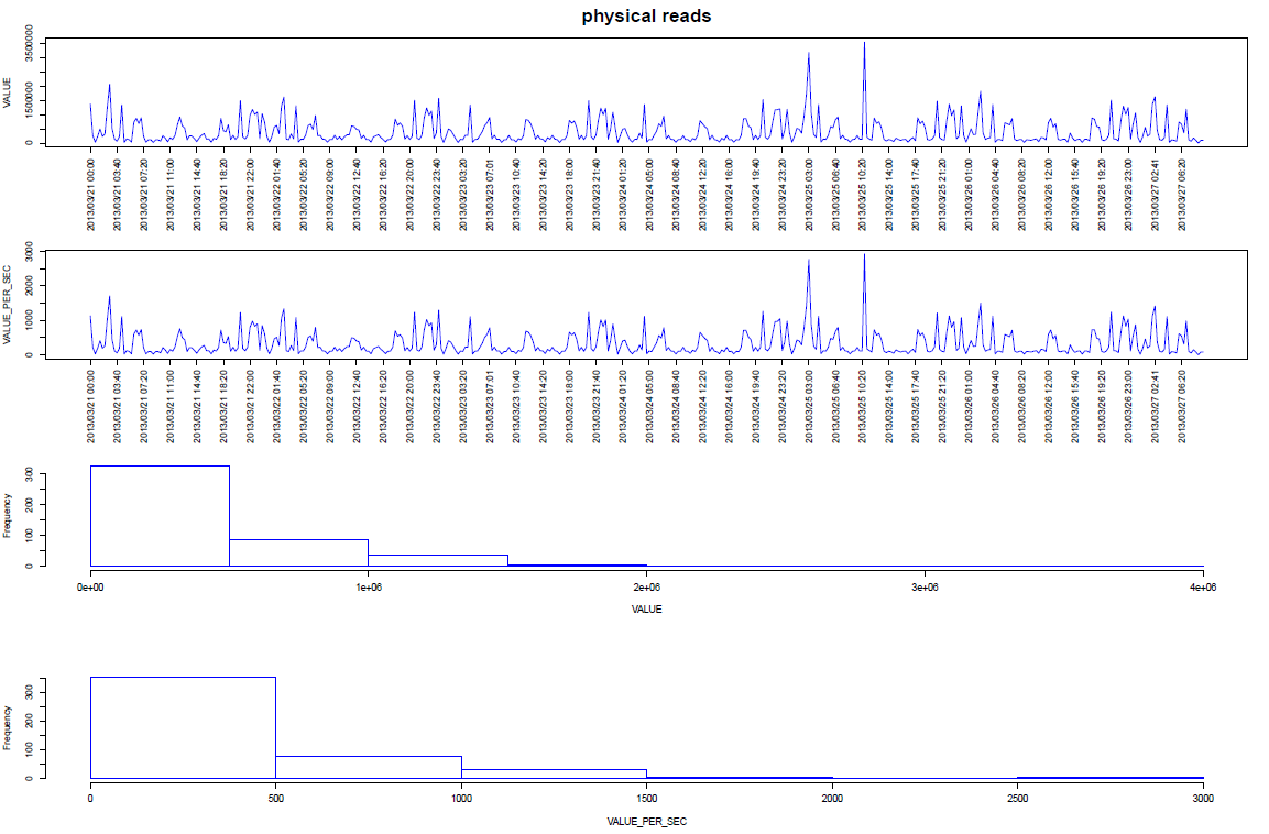 and the physical_reads pdf file will be generated as well.
As you can see, you are prompted for:
- jdbc thin “like” details to connect to the database (You can launch the R script outside the host hosting the database)
- oracle system user password
- The statistic we want to focus on
- Number of days to go back as the time frame starting point
- Number of days to go back as the time frame ending point
Remarks:
- You need to purchase the Diagnostic Pack in order to be allowed to query the AWR repository.
- If the script has been launched with X11 not working properly, you’ll get:
Loading required package: methods
Loading required package: DBI
Loading required package: rJava
[1] "Not able to display, so only pdf generation..."
Warning message:
In x11(width = 15, height = 10) :
  unable to open connection to X11 display ''
[1] 11
Please enter any key to exit:
But the script takes care of it and the pdf file will be generated anyway.
Conclusion:
We are able to display graphically AWR historical metrics for a particular statistic over a period of time with the help of a single script named: graph_awr_sysstat.r (You can download it from this repository).
If you don’t have R installed:
- you can use the sql provided at the beginning of this post to get at least a “text” view of the historical metrics.
- Install it :-) (See “Getting Starting” from this link)
Update: If you want to see the same metrics in real time then you could have a look to this post.