In this post I will provide a way to retrieve wait events metrics from AWR and to display graphically those metrics thanks to R over a period of time.
Why R ?: Because R is a powerful tool for statistical analysis with graphing and plotting packages built in. Furthermore, R can connect to Oracle via a JDBC package which makes importing data very easy.
So, for a particular wait event, I’ll retrieve from the dba_hist_system_event view:
- TIME_WAITED_MS: Time waited in ms between 2 snaps
- TOTAL_WAITS: Number of waits between 2 snaps
- MS_PER_WAIT: Avg wait time in ms between 2 snaps
As those metrics are cumulative ones, I need to compute the difference between 2 snaps that way:
SQL> !cat check_awr_event.sql
set linesi 220;

alter session set nls_date_format='DD-MM-YYYY HH24:MI:SS';

col BEGIN_INTERVAL_TIME format a28
col event_name format a40
col WAIT_CLASS format a20
set pagesi 999

select distinct(WAIT_CLASS) from v$system_event;

select e.WAIT_CLASS,e.event_name,s.begin_interval_time,e.TOTAL_WAITS,e.TIME_WAITED_MS,e.TIME_WAITED_MS / TOTAL_WAITS "MS_PER_WAIT"
from
(
select instance_number,snap_id,WAIT_CLASS,event_name,
total_waits - first_value(total_waits) over (partition by event_name order by snap_id rows 1 preceding) "TOTAL_WAITS",
(time_waited_micro - first_value(time_waited_micro) over (partition by event_name order by snap_id rows 1 preceding))/1000 "TIME_WAITED_MS"
from
dba_hist_system_event
where
WAIT_CLASS like nvl('&WAIT_CLASS',WAIT_CLASS)
and event_name like nvl('&event_name',event_name)
and instance_number = (select instance_number from v$instance)
) e, dba_hist_snapshot s
where e.TIME_WAITED_MS > 0
and e.instance_number=s.instance_number
and e.snap_id=s.snap_id
and s.BEGIN_INTERVAL_TIME >= trunc(sysdate-&sysdate_nb_day_begin_interval+1)
and s.BEGIN_INTERVAL_TIME <= trunc(sysdate-&sysdate_nb_day_end_interval+1) order by 1,2,3;
I use the “partition by event_name order by snap_id rows 1 preceding” to compute the difference between snaps per event.
The output is like:
SQL> @check_awr_event.sql

Session altered.

WAIT_CLASS
--------------------
Administrative
Application
Commit
Concurrency
Configuration
Idle
Network
Other
System I/O
User I/O

10 rows selected.

Enter value for wait_class:
old  10: WAIT_CLASS like nvl('&WAIT_CLASS',WAIT_CLASS)
new  10: WAIT_CLASS like nvl('',WAIT_CLASS)
Enter value for event_name: db file sequential read
old  11: and event_name like nvl('&event_name',event_name)
new  11: and event_name like nvl('db file sequential read',event_name)
Enter value for sysdate_nb_day_begin_interval: 7
old  17: and s.BEGIN_INTERVAL_TIME >= trunc(sysdate-&sysdate_nb_day_begin_interval+1)
new  17: and s.BEGIN_INTERVAL_TIME >= trunc(sysdate-7+1)
Enter value for sysdate_nb_day_end_interval: 0
old  18: and s.BEGIN_INTERVAL_TIME <= trunc(sysdate-&sysdate_nb_day_end_interval+1) order by 1,2,3
new  18: and s.BEGIN_INTERVAL_TIME <= trunc(sysdate-0+1) order by 1,2,3

WAIT_CLASS           EVENT_NAME                               BEGIN_INTERVAL_TIME          TOTAL_WAITS TIME_WAITED_MS MS_PER_WAIT
-------------------- ---------------------------------------- ---------------------------- ----------- -------------- -----------
User I/O             db file sequential read                  20-MAR-13 12.00.45.270 AM         286608     271639.345  .947773073
User I/O             db file sequential read                  20-MAR-13 12.20.49.821 AM          32759     125296.732  3.82480332
User I/O             db file sequential read                  20-MAR-13 12.40.54.540 AM           4404       8946.577  2.03146617
User I/O             db file sequential read                  20-MAR-13 01.00.58.981 AM           3617       4737.182   1.3096992
User I/O             db file sequential read                  20-MAR-13 01.20.03.039 AM          22624      94671.254  4.18454977
User I/O             db file sequential read                  20-MAR-13 01.40.07.163 AM          94323     181118.282  1.92019213
User I/O             db file sequential read                  20-MAR-13 02.00.11.636 AM         119458     317204.205  2.65536176
User I/O             db file sequential read                  20-MAR-13 02.20.16.040 AM          81720     212678.865  2.60253139
User I/O             db file sequential read                  20-MAR-13 02.40.20.827 AM          61664     120446.947   1.9532782
User I/O             db file sequential read                  20-MAR-13 03.00.25.531 AM          92493     110715.902  1.19701926
User I/O             db file sequential read                  20-MAR-13 03.20.29.923 AM           2692       6102.149  2.26677155
So if you use this sql, you’ll be able to see for a particular event its historical behaviour. That’s fine and I used it a lot of times.
But I like also to have a graphical view of what’s going on, and that is exactly where R comes into play.
I created a R script named: graph_awr_event.r (You can download it from this repository) that provides:
- A graph for the TIME_WAITED_MS metric over the period of time
- A graph for the NB_WAITS metric over the period of time
- A graph for the MS_PER_WAIT metric over the period of time
- A graph for the Histogram of MS_PER_WAIT over the period of time
- A pdf file that contains those graphs
- A text file that contains the metrics used to build the graphs
The graphs will come from both outputs (X11 and the pdf file). In case the X11 environment does not work, the pdf file is generated anyway.
As a graphical view is better to understand, let’s have a look how it works and what the display is:
For example, let’s focus on the “db file sequential read” wait event over the last 7 days that way:
./graph_awr_event.r
Building the thin jdbc connection string....

host ?: bdt_host
port ?: 1521
service_name ?: bdt
system password ?: XXXXXXXX
Display which event (no quotation marks) ?: db file sequential read
Please enter nb_day_begin_interval: 7
Please enter nb_day_end_interval: 0
Loading required package: methods
Loading required package: DBI
Loading required package: rJava
[1] 11
Please enter any key to exit:
The output will be like:
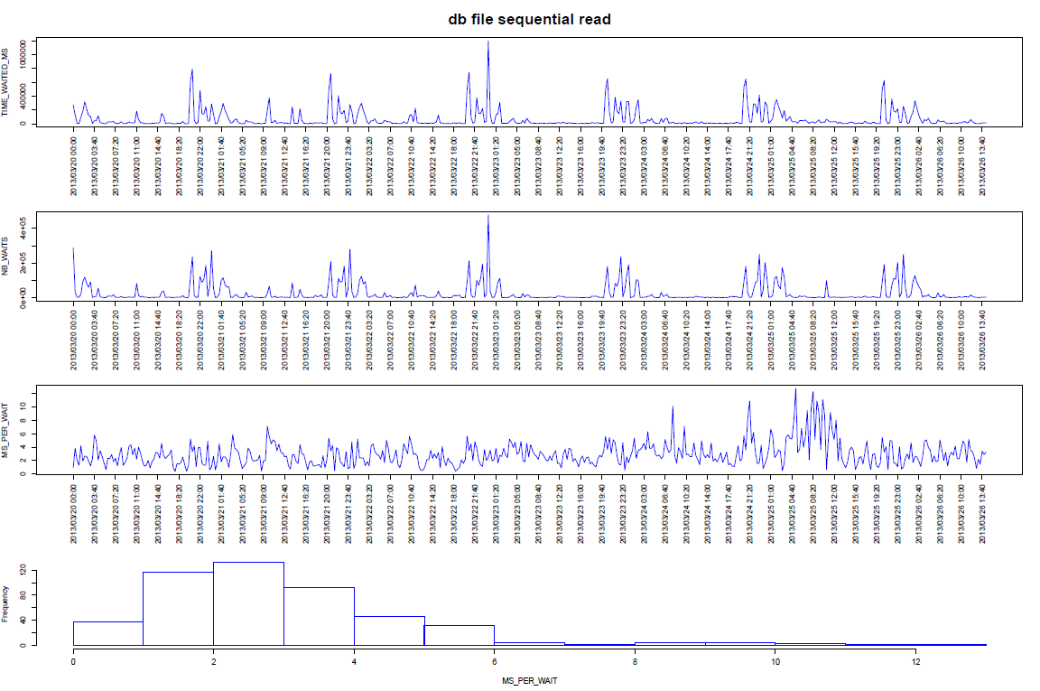
and the db_file_sequential_read pdf file will be generated as well.
As you can see, you are prompted for:
- jdbc thin “like” details to connect to the database (You can launch the R script outside the host hosting the database)
- oracle system user password
- The wait event we want to focus on
- Number of days to go back as the time frame starting point
- Number of days to go back as the time frame ending point
Remarks:
- You need to purchase the Diagnostic Pack in order to be allowed to query the AWR repository.
- If the script has been launched with X11 not working properly, you’ll get:
Loading required package: methods
Loading required package: DBI
Loading required package: rJava
[1] "Not able to display, so only pdf generation..."
Warning message:
In x11(width = 15, height = 10) :
  unable to open connection to X11 display ''
[1] 11
Please enter any key to exit:
But the script takes care of it and the pdf file will be generated anyway.
Conclusion:
We are able to display graphically AWR historical metrics for a particular wait event over a period of time with the help of a single script named: graph_awr_event.r (You can download it from this repository).
If you don’t have R installed:
- you can use the sql provided at the beginning of this post to get at least a “text” view of the historical metrics.
- Install it ;-) (See “Getting Starting” from this link)
Updates:
- You can do the same with system statistics (see Retrieve and visualize system statistics from AWR with R)
- You can do the same in real time (see Retrieve and visualize in real time wait events metrics with R)